Input format

To demonstrate the python data types required to represent the input, we use the utility function make_data which returns randomly generated data that we will use for this example. See the function’s documentation for more information regarding its parameters.

from occuspytial.utils import make_data

Q, W, X, y, true_alpha, true_beta, true_tau, true_z = make_data(random_state=0)

The Gibbs samplers expect (at the minimum) as input the design matrix for occupancy covariates, the design matrices for detection covariates, the detection/non-detection data and the spatial precision matrix of the ICAR spatial random effects.

Q represents the spatial precision matrix and can either be scipy’s sparse matrix object or a numpy array. If a numpy array is used, the sampler convert it to a sparse matrix. It is advised that Q be in sparse format since the format is more memory efficient.

Q

<150x150 sparse matrix of type '<class 'numpy.float64'>'
        with 1204 stored elements in COOrdinate format>

Detection/non-detection observed data (y) should be depresented using a dictionary whose key is the site number (only sites that were surveyed) and value is a numpy array whose elements are 1’s (if the species is detected on that visit) and 0’s. The length of the array should represent the number of visits for that site.

y.keys()

dict_keys([15, 130, 33, 114, 7, 105, 121, 148, 27, 103, 40, 106, 1, 90, 69, 8, 29, 76, 101, 24, 75, 112, 142, 77, 85, 51, 43, 30, 47, 139, 93, 99, 45, 26, 55, 131, 79, 122, 115, 120, 54, 125, 117, 36, 28, 57, 22, 37, 78, 5, 109, 95, 49, 17, 4, 62, 13, 104, 108, 118, 135, 137, 3, 32, 18, 116, 100, 53, 65, 80, 91, 86, 42, 2, 14])

y[15]  # 4 visits in site 15 with no detection of the species on

array([0, 0, 0, 0])

Similarly, the detection covariates (W) are represented by a dictionary whose key is the site number (only sites that were surveyed) and value is a 2d numpy array representing the design matrix of the detection covariates of that site.

W[15]

array([[ 1.        , -0.54769293,  1.19683385],
       [ 1.        ,  0.56049534,  0.06091067],
       [ 1.        ,  1.49854722,  0.39848634],
       [ 1.        ,  1.74023235, -1.3585544 ]])

Occupancy covariates (X) are represented by a design matrix which is a 2d numpy array.

X[:5]  # occupancy design matrix for the first 5 sites

array([[ 1.        ,  1.9343916 ,  0.41607945],
       [ 1.        ,  1.57410391, -0.88706203],
       [ 1.        , -1.4857609 ,  0.31065634],
       [ 1.        , -0.72944554,  0.27830849],
       [ 1.        , -1.36270245,  0.22016475]])

The rest of the output from make_data are the simulated true values for spatial occupancy model parameters.

print('alpha: ', true_alpha, '\n', 'beta: ', true_beta, '\n', 'tau: ', true_tau, '\n', 'z (occupancy state): ', true_z)

alpha:  [-0.62578191 -0.76973348  0.89920592]
 beta:  [ 0.16133415 -1.4298573  -1.29695223]
 tau:  0.6567761989615925
 z (occupancy state):  [0 1 1 1 1 1 1 0 1 1 0 1 0 0 1 0 0 1 1 0 1 0 0 1 0 0 1 1 0 1 1 0 0 0 0 0 0
 1 1 0 0 1 0 1 1 0 0 1 1 0 1 0 0 1 1 1 1 1 0 1 1 1 1 1 0 0 1 0 0 0 1 1 1 0
 0 1 0 1 1 1 0 0 1 0 1 1 0 0 0 0 1 1 0 1 0 0 0 0 1 0 0 1 1 1 1 1 0 0 0 1 1
 0 1 1 1 1 0 0 1 1 0 0 1 0 1 0 1 1 1 1 1 1 0 1 1 1 0 1 1 0 0 1 0 0 1 1 1 1
 1 1]

Sampling example

This section contains basic examples of how to use the available samplers.

Gibbs sampling

Here we show how to use the Gibbs sampler presented in Clark & Altwegg (2019) using OccuSpytial’s sampler API. The name of the class implementing this sampler is LogitRSRGibbs

import numpy as np

from occuspytial import LogitRSRGibbs
from occuspytial.utils import make_data

# generate fake data with 500 sites in total
Q, W, X, y, true_alpha, true_beta, true_tau, true_z = make_data(500, tau_range=(0.1, 0.5), random_state=0)

Lets print out the true values of the parameters of interest.

print('alpha: ', true_alpha, '\n', 'beta: ', true_beta, '\n', 'tau: ', true_tau)

alpha:  [-1.8990662   1.46050246  0.35355792]
 beta:  [ 0.45288262 -0.50514168  0.10059925]
 tau:  0.36959287108483785

rsr = LogitRSRGibbs(Q, W, X, y, random_state=10)
rsr_samples = rsr.sample(2000, burnin=1000, chains=2)
# The progressbar is on by default, but Jupyter notebook only displays it on the console
# so it is not visible in the output cell of this notebook unlike if we are working on the console.

The output of the sample method is an instance of the PosteriorParameter class and inference of the samples obtained are done via the instance stored in the variable rsr_samples. We can display the summary table using the summary attribute.

rsr_samples.summary

	mean	sd	hdi_3%	hdi_97%	mcse_mean	mcse_sd	ess_bulk	ess_tail	r_hat
alpha[0]	-2.090	0.072	-2.224	-1.959	0.004	0.003	280.0	607.0	1.01
alpha[1]	1.643	0.063	1.517	1.760	0.004	0.003	291.0	678.0	1.02
alpha[2]	0.437	0.042	0.348	0.510	0.002	0.001	659.0	1338.0	1.00
beta[0]	0.415	0.251	-0.014	0.929	0.018	0.013	185.0	271.0	1.01
beta[1]	-0.705	0.201	-1.082	-0.328	0.014	0.010	200.0	392.0	1.01
beta[2]	-0.153	0.190	-0.500	0.220	0.014	0.010	196.0	454.0	1.01
tau	0.030	0.012	0.011	0.051	0.001	0.001	75.0	249.0	1.06

To access the individual parameters we can use the the parameter’s name as the key.

rsr_samples['alpha']

array([[[-2.01705032,  1.65307598,  0.401219  ],
        [-2.14701198,  1.64676912,  0.43997882],
        [-2.01331818,  1.58390992,  0.39207318],
        ...,
        [-2.0125808 ,  1.62231449,  0.45280794],
        [-1.96998293,  1.62743685,  0.39180286],
        [-2.05031195,  1.67996656,  0.47238301]],

       [[-2.00735185,  1.65148581,  0.44014908],
        [-2.02527985,  1.568106  ,  0.39224504],
        [-2.00480733,  1.54194479,  0.32078477],
        ...,
        [-2.09342836,  1.57293681,  0.46988205],
        [-2.06795498,  1.61602514,  0.48115473],
        [-2.02151848,  1.60897632,  0.45971322]]])

Since we generated 2 chains, alpha parameter array is three dimensional; where the first dimension is the chain index, the second dimension is the length of the post-burnin samples, and the third dimension is the size of the parameter (in elements).

rsr_samples['alpha'].shape

(2, 1000, 3)

LogitRSRGibbs expects the prior distributions for alpha and beta to be normal distributed, and the prior for tau to be Gamma distributed. We can pass custom values for the hyperparameters of these priors through the hparams dictionary parameter during instantiation of the class instance. More details on legal keys and values can be found in the docstring of the class.

a_size = true_alpha.shape[0]
b_size = true_beta.shape[0]
hypers = {
    'a_mu': np.ones(a_size),  # alpha mean is an array of 1's
    'a_prec': np.eye(a_size) / 1000,  # alpha precision matrix (inverse of covariance) is diagonal matrix with entries (1/1000)
    'b_mu': np.ones(b_size),
    'b_prec': np.eye(a_size) / 1000,
    'tau_rate': 2,  # tau's rate parameter for the prior gamma distribution
    'tau_shape': 2,  # tau's shape parameter
}
rsr_hp = LogitRSRGibbs(Q, W, X, y, hparams=hypers, random_state=10)
rsrhp_samples = rsr_hp.sample(2000, burnin=1000, chains=2)
rsrhp_samples.summary

	mean	sd	hdi_3%	hdi_97%	mcse_mean	mcse_sd	ess_bulk	ess_tail	r_hat
alpha[0]	-2.169	0.072	-2.315	-2.042	0.016	0.011	21.0	103.0	1.08
alpha[1]	1.592	0.064	1.467	1.705	0.014	0.010	21.0	252.0	1.08
alpha[2]	0.421	0.044	0.334	0.499	0.004	0.003	101.0	1203.0	1.03
beta[0]	31.860	11.925	10.092	50.254	7.436	6.006	3.0	19.0	2.13
beta[1]	-40.554	9.686	-53.542	-20.947	5.832	4.661	3.0	12.0	1.63
beta[2]	-19.367	4.297	-26.079	-10.843	2.021	1.533	5.0	13.0	1.35
tau	0.000	0.000	0.000	0.000	0.000	0.000	67.0	808.0	1.03

As we can see the MCMC chain did not converge in just 2000 samples with the provided hyper-parameter values. We can either improve the estimates by using a much longer chain or use better starting values in the sample method via the start parameter.

Visualizing posterior samples

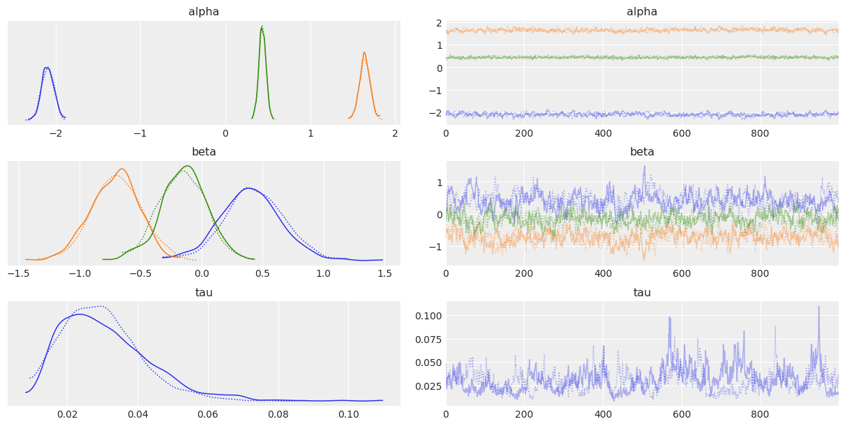
rsr_samples instance allows for convenient visualization of posterior samples of the parameters of interest. This functionality uses arviz as a backend. We can plot the traces and densities as follows:

rsr_samples.plot_trace()

array([[<AxesSubplot:title={'center':'alpha'}>,
        <AxesSubplot:title={'center':'alpha'}>],
       [<AxesSubplot:title={'center':'beta'}>,
        <AxesSubplot:title={'center':'beta'}>],
       [<AxesSubplot:title={'center':'tau'}>,
        <AxesSubplot:title={'center':'tau'}>]], dtype=object)

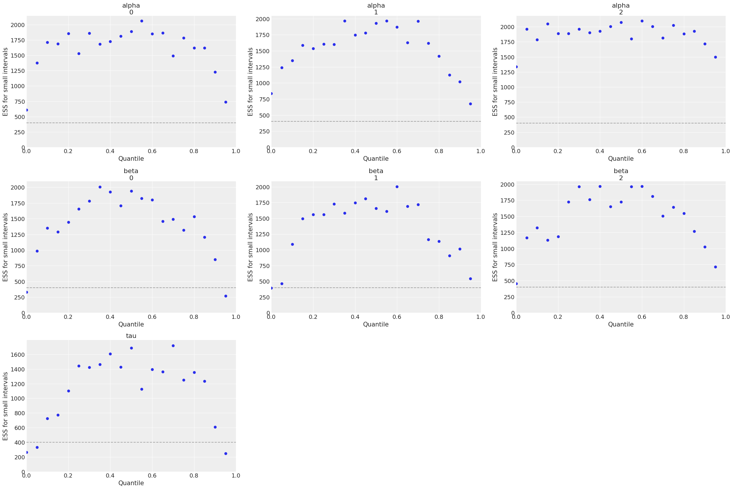
Parameters can be passed into the plot_trace method to configure the output plot. See arviz’s API reference for valid input. Similarly, the Effective Sample Size (ESS) can be visualized as follows:

rsr_samples.plot_ess()

array([[<AxesSubplot:title={'center':'alpha\n0'}, xlabel='Quantile', ylabel='ESS for small intervals'>,
        <AxesSubplot:title={'center':'alpha\n1'}, xlabel='Quantile', ylabel='ESS for small intervals'>,
        <AxesSubplot:title={'center':'alpha\n2'}, xlabel='Quantile', ylabel='ESS for small intervals'>],
       [<AxesSubplot:title={'center':'beta\n0'}, xlabel='Quantile', ylabel='ESS for small intervals'>,
        <AxesSubplot:title={'center':'beta\n1'}, xlabel='Quantile', ylabel='ESS for small intervals'>,
        <AxesSubplot:title={'center':'beta\n2'}, xlabel='Quantile', ylabel='ESS for small intervals'>],
       [<AxesSubplot:title={'center':'tau'}, xlabel='Quantile', ylabel='ESS for small intervals'>,
        <AxesSubplot:>, <AxesSubplot:>]], dtype=object)

For more information about other available plots, see documentation of PosteriorParameter class.